

Quick image scaling by 2
In a preceding article ([1]) I presented an adaptation of the linear Bresenham algorithm to scale images with a quality that approximates that of linear interpolation. I called this algorithm "smooth Bresenham scaling". In the article, I noted that the scale factor should lie within the range of 50% to 200% for the routine to work correctly. Then, it went on to suggest that, if you need a scaling factor outside that range, you can use a separate algorithm that scales an image up or down by a factor of 2 and then use smooth Bresenham to scale to the final size. Scaling by a factor of 2 is the topic of this article.
This article and the preceding one could be seen as a single article cut in two parts: it is their combined use that results in a general purpose, fast image scaling algorithm with adequate quality. Both articles rely on an average() function that is covered in a separate article [2].
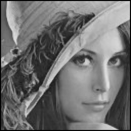
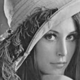
Like the previous article, the algorithms described here process colour images in a single pass without unpacking and repacking pixels into separate RGB channels. Although the example images in this article are all grey scale (single channel), the same algorithms are suitable for three-channel colour images and for palette-indexed images.
A simple 1/2× image scaler
One of the simplest ways to halve the resolution of a picture is to replace each quad of four pixels by one pixel with is the average of the four pixels. Sampling theory calls this a "box filter"; in my experience, the box filter gives good quality when minifying an image by an integral factor.
When the average of four pixels is easy to calculate, by all means do so. If it is harder to calculate, such as with palette indexed images, you may opt to use the average() function (see [2]) three times in succession, as is done in the snippet below.
template<class PIXEL>
void ScaleMinifyByTwo(PIXEL *Target, PIXEL *Source, int SrcWidth, int SrcHeight)
{
  int x, y, x2, y2;
  int TgtWidth, TgtHeight;
  PIXEL p, q;

  TgtWidth = SrcWidth / 2;
  TgtHeight = SrcHeight / 2;
  for (y = 0; y < TgtHeight; y++) {
    y2 = 2 * y;
    for (x = 0; x < TgtWidth; x++) {
      x2 = 2 * x;
      p = average(Source[y2*SrcWidth + x2], Source[y2*SrcWidth + x2 + 1]);
      q = average(Source[(y2+1)*SrcWidth + x2], Source[(y2+1)*SrcWidth + x2 + 1]);
      Target[y*TgtWidth + x] = average(p, q);
    } /* for */
  } /* for */
}
I have written the code in above snippet for clarity more than to serve as production code. One obvious optimization is to avoid calculating the same values over and over again: the expressions y2*SrcWidth, (y2+1)*SrcWidth and y*TgtWidth remain constant in the inner loop and should be substituted by pre-computed variables. Perhaps you can trust your compiler to do this optimization for you.
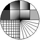
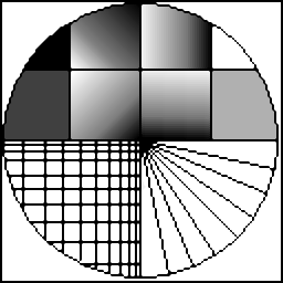
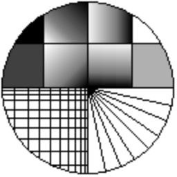
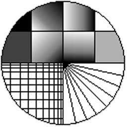
From the example images shown below, it is apparent that the box filter is equivalent to linear interpolation with this particular scale factor. The box filter (and the bilinear interpolator) perform better than the bicubic interpolator when minifying: the resulting images of the bicubic interpolator are blurred, as you can see from the scaled "line graphics" images.
 Original picture |
 50% - Box filter |
 50% - Bilinear interpolation |
 50% - Bicubic interpolation |
 Original picture |
 50% - Box filter |
 50% - Bilinear interpolation |
 50% - Bicubic interpolation |
An edge-sensitive directionally averaging 2× image scaler
Among the more popular algorithms for enlarging a bitmapped image are pixel replication and bilinear interpolation; these algorithms are quick and simple to implement. The pixel replication algorithm simply copies the nearest pixel (nearest neighbour sampling). As a result, the algorithm is prone to blockiness, which is especially visible along the edges. Bilinear interpolation is at the other extreme, it takes the (linearly) weighted average of the four nearest pixels around the destination pixel. This causes gradients to be fluently interpolated, and edges to be blurred. Several other algorithms use different weightings and/or more pixels to derive a destination pixel from a surrounding set of source pixels.
The reasoning behind these algorithms is that the value of a destination pixel must be approximated from the values of the surrounding source pixels. But you can do better than just to take the distances to the surrounding pixels and a set of fixed weight factors stored in a matrix. Directional interpolation is a method that tries to interpolate along edges in a picture, not across them.
My interest in directional interpolation was spurred by two papers. In [6] the authors use polynomial interpolation with gradient-dependent weights. To calculate the gradients, the paper applies a pair of Sobel masks on every source pixel taking part in the interpolation. The algorithm in [7] splits a source pixel into four target pixels in one pass, considering eight additional surrounding pixels (nine source pixels in total). By applying a matrix with pre-computed weights for every relation between the nine pixels, the value of each of the four target pixels is calculated.
The algorithm in [6] has fairly simple operations on every source pixel that it considers for each target pixel, but it considers a big set of source pixels. This is a major performance bottleneck. The other paper ([7]) uses a few surrounding pixels, and calculates four destination pixels in one pass, but the amount of arithmetic required for the calculation makes it unsuitable for real-time scaling. Neither algorithm is easily adapted to colour images; a colour image is regarded as a 3-channel image where each channel must be resized individually.
The idea, then, is to combine concepts from the two papers, but at a lower cost: simple operations on few source pixels per target pixel.
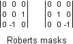
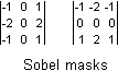
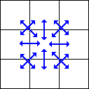
A directionally interpolation algorithm requires that you find the edges first, or rather, that you determine the direction of the gradient at every pixel. While the paper [6] uses only the magnitude of the gradient, [7] also considers its direction, to its advantage. Simple edge detectors that are suitable to find the gradient (magnitude and direction), are pairs of Roberts masks or Sobel masks. In the figure below, the Roberts masks are put in 3×3 matrices, but, as you can see, calculating the value of one mask involves just one subtraction. Either Roberts mask detects an edge in a diagonal direction. From the two values, you can calculate both the direction of the gradient and the "steepness" of the gradient. The other figure below shows a pair of Sobel masks; one Sobel mask detects an edge in the horizontal or vertical direction and, like the Roberts masks, both Sobel masks are combined for the complete gradient information. Given the direction of the gradient, I could then choose an appropriate directional interpolator. These interpolators are just linear, not bilinear.
Roberts masks are known to be sensitive to noise: they tend to detect an edge where there is no real edge. Since my goal is to simply choose between interpolators, I figured that choosing a directional interpolator on a pixel where there is no edge, would not matter much. I had not foreseen, however, that the sensitivity of Roberts masks might also result in returning the wrong direction of the gradient in the presence of an edge. This flaw makes Roberts masks unsuitable for directional interpolation. Sobel masks are generally considered to be robust while still being simple. They consider three times as many source pixels, so their estimate of the gradient direction should be significantly more accurate. To my surprise, however, I found that Sobel masks would completely miss a horizontal or vertical line with a width of one pixel that runs through the middle of the masks. A one-pixel wide diagonal line on an angle of 45° or 135° is also missed. Both in my line graphic test image and in the Lena picture, this proved to cause severe "noise" due to wrongly determined gradient directions. I experimented with combinations of Roberts and Sobel masks, but these were unsuccessful.
 The flaw in the above approach is that a region of 9 pixels is too small to
determine the direction of an edge running through the middle pixel, which
the authors of [6] had probably encountered as well.
Instead of selecting a larger edge detection kernel, however, I decided to split
each source pixel into four target pixels, like in [7],
and finding the interpolation partner per target pixel (so one source pixel
may have four different interpolation partners). This new approach calculates
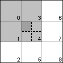
four gradients for each source pixel. The figure at the right of this paragraph
represents nine pixels from the source image. To calculate the target pixel for
the upper left quadrant for the middle source pixel, the algorithm considers
the source pixels 0, 1, 3 and 4. It finds the direction with the lowest gradient
in this region of four source pixels and uses that to select the interpolation
candidates. While I could have used a pair of Roberts masks to get the gradient
direction, simply selecting the minimum distance between any of the four
possible pairs of the four source pixels under consideration was more effective
and actually simpler to implement.
The flaw in the above approach is that a region of 9 pixels is too small to
determine the direction of an edge running through the middle pixel, which
the authors of [6] had probably encountered as well.
Instead of selecting a larger edge detection kernel, however, I decided to split
each source pixel into four target pixels, like in [7],
and finding the interpolation partner per target pixel (so one source pixel
may have four different interpolation partners). This new approach calculates
four gradients for each source pixel. The figure at the right of this paragraph
represents nine pixels from the source image. To calculate the target pixel for
the upper left quadrant for the middle source pixel, the algorithm considers
the source pixels 0, 1, 3 and 4. It finds the direction with the lowest gradient
in this region of four source pixels and uses that to select the interpolation
candidates. While I could have used a pair of Roberts masks to get the gradient
direction, simply selecting the minimum distance between any of the four
possible pairs of the four source pixels under consideration was more effective
and actually simpler to implement.
The algorithm is conceptually simple: of all source pixels under consideration, it interpolates between the pair of pixels with the lowest difference. The upper left target pixel may be:
- interpolated between source pixels 4 and 1,
- interpolated between source pixels 4 and 3,
- interpolated between source pixels 4 and 0 or
- interpolated between source pixel 4 and the average of source pixels 1 and 3.
The first step is to calculate the differences between the pairs of source pixels 4-1, 4-3, 4-0 and 3-1. Actually, I am not interested in the sign of the differences, just the distances. The algorithm determines the minimum distance and chooses the appropriate interpolator. Interpolation, in this particular context, just means (unweighted) averaging; so in the case of first interpolator, the colour of target pixel is the halfway between of source pixels 4 and 1.
The code snippet below computes the "upper left" target pixel for a source pixel at coordinate (x, y). Using a similar procedure, one obtains the other three target pixels for this source pixel.
#define ABS(a)          ( (a) >= 0 ? (a) : -(a) )

      p = Source[y*SrcWidth + x];

      /* target pixel in North-West quadrant */
      p1 = Source[(y-1)*SrcWidth + x];      /* neighbour to the North */
      p2 = Source[y*SrcWidth + (x-1)];      /* neighbour to the West */
      p3 = Source[(y-1)*SrcWidth + (x-1)];  /* neighbour to the North-West */
      d1 = ABS( colordiff(p, p1) );
      d2 = ABS( colordiff(p, p2) );
      d3 = ABS( colordiff(p, p3) );
      d4 = ABS( colordiff(p1, p2) );        /* North to West */

      /* find minimum */
      min = d1;
      if (min > d2) min = d2;
      if (min > d3) min = d3;
      if (min > d4) min = d4;

      /* choose interpolator */
      y2 = 2 * y;
      x2 = 2 * x;
      if (min == d1)
        Target[y2*TgtWidth+x2] = average(p, p1);        /* North */
      else if (min == d2)
        Target[y2*TgtWidth+x2] = average(p, p2);        /* West */
      else if (min == d3)
        Target[y2*TgtWidth+x2] = average(p, p3);        /* North-West */
      else /* min == d4 */
        Target[y2*TgtWidth+x2] = average(p, average(p1, p2));/* North to West */
In an early implementation, the last interpolator just set the target pixel to the average of source pixels 1 and 3. In testing, I found that I obtained better results by averaging with source pixel 4 afterwards too. Due to the two consecutive averaging operations, the target pixel's colour is ultimately set to ½S4 + ¼S1 + ¼S3 (where Si stands for "source pixel i").
The images below compare the directionally averaging algorithm to bilinear and bicubic interpolation. Directional interpolation achieves sharper results than both bilinear and bicubic interpolation. Note that the original "line graphics" picture was intentionally created without anti-aliasing. It is to be expected that the output contains "jaggies" too.
Original picture |
 200% - Directional averaging |
 200% - Bilinear interpolation |
 200% - Bicubic interpolation |
Original picture |
 200% - Directional averaging |
 200% - Bilinear interpolation |
 200% - Bicubic interpolation |
Quick, approximate colour distances
For the directionally averaging scaling algorithm to be feasible, you must have a way to determine the difference between the colours of two pixels. In the code snippet for magnifying by 2, this is hidden in the colordiff() function. This "pixel difference" calculation is also likely to become the performance bottleneck of the application, which is why I will give it a little more attention.
For grey scale pixels, calculating the pixel distance is as simple as taking the absolute value of the subtraction of a pair of pixels. The SIMD instructions ("single instructions, multiple data", previously known as MMX) of the current Intel Pentium processors allow you to obtain absolute values of four signed 16-bit values in parallel, using only a few instructions. For example code, see [4].
When checking the references for this article, I noticed that the Intel Application note "AP-563" ([4]) was apparently no longer available on the Intel website. Therefore, I will spend a few words on the "trick".
In two's complement arithmetic, to negate an integer, you flip all bits and add one. To toggle all bits, you can use the NOT instruction, or you can XOR by -1. Adding 1 is of course equivalent to subtracting -1. Everything falls together when you find an easy way to set a register to -1 or zero, based on the sign bit of the source value. The CWD and the SAR instructions can do this. To get the absolute value of a value in AX, you can use:The SIMD instructions allow you to process four 16-bit values at a time.cwd ; dx = -1 iff ax < 0, or 0 iff ax >= 0 xor ax, dx ; invert ax iff dx is -1 sub ax, dx ; increment ax iff dx = -1
For 24-bit true colour images, you have several options to calculate the pixel distance:
- Use an accurate colour distance measure, such as the Euclidean vector length in 3-dimensional RGB space. This is probably too slow for our purposes, however, and it is also far more accurate than we need.
- Convert both pixels to grey scale, then calculate the distance between the grey scale values. Depending on how you calculate the grey scale equivalents of colour pixels, this may still be quite a slow procedure.
- Calculate the differences for all three channels separately and take the largest of these three values.
- Interleave the bits for the red, green and blue channel values and determine the difference between two interleaved values.
I propose the method listed last: bit interleaving. Bit interleaving has been widely used to create (database) indices and to find clusters in spatial data sets, specifically when the data set is represented in a quad- or octree. Applying bit interleaving to the RGB colour cube to find approximate colour differences is a straightforward extension, see [3].
Bit interleaving is actually a simple trick where an RGB colour that stored in three bytes with an encoding like:
R7R6R5R4R3R2R1R0 - G7G6G5G4G3G2G1G0 - B7B6B5B4B3B2B1B0is transformed to:
G7R7B7G6R6B6G5R5 - B5G4R4B4G3R3B3G2 - R2B2G1R1B1G0R0B0
The new encoding groups bits with the same significance together and the subtraction between two of these interleaved values is thus a fair measure of the distance between the colours. To calculate the interleaved encoding quickly, one uses a precalculated lookup table that maps an input value (in the range 0 – 255) to the encoding:
A7A6A5A4A3A2A1A0to:
0 0 A70 0 A60 0 - A50 0 A40 0 A30 - 0 A20 0 A10 0 A0With this table, you need only three table lookup's (for the red, green and blue channels), two bit shifts and two bitwise "OR" instructions to do the full conversion. See the code snippet below for an implementation; the code assumes that you call the function CreateInterleaveTable() during the initialization of your application.
typedef struct __s_RGB {
  unsigned char r, g, b;
} RGB;

static long InterleaveTable[256];

void CreateInterleaveTable(void)
{
  int i,j;
  long value;

  for (i = 0; i < 256; i++) {
    value = 0L;
    for (j = 0; j < 8; j++)
      if (i & (1 << j))
        value |= 1L << (3*j);
    InterleaveTable[i] = value;
  } /* for */
}

/* 24-bit RGB (unpacked pixel) */
long InterleavedValue(RGB color)
{
  return (InterleaveTable[color.g] << 2) |
         (InterleaveTable[color.r] << 1) |
          InterleaveTable[color.b];
}
Optimizations and other notes
 As mentioned earlier, the pixel difference algorithm is likely to become the
limiting factor in the routine's performance. One implementation-specific
optimization trick was already mentioned: exploit parallelism by using SIMD
instructions. There are also a couple of algorithmic optimizations that help. In
the code snippet for magnifying by 2, we can count that
we need to calculate four pixel distances per target pixel. For four target
pixels per source pixel, that amounts to 16
pixel distances. The first opportunity for optimization is to recognize that
there is overlap in the neighbouring pixels used for each of the target pixels,
see the figure 6 at the right. When grouping the calculations of all
pixel distances for one source pixel (four target pixels), one sees that there
are 12 unique pixel distances that must be calculated —already a 25% savings
from the original 16.
As mentioned earlier, the pixel difference algorithm is likely to become the
limiting factor in the routine's performance. One implementation-specific
optimization trick was already mentioned: exploit parallelism by using SIMD
instructions. There are also a couple of algorithmic optimizations that help. In
the code snippet for magnifying by 2, we can count that
we need to calculate four pixel distances per target pixel. For four target
pixels per source pixel, that amounts to 16
pixel distances. The first opportunity for optimization is to recognize that
there is overlap in the neighbouring pixels used for each of the target pixels,
see the figure 6 at the right. When grouping the calculations of all
pixel distances for one source pixel (four target pixels), one sees that there
are 12 unique pixel distances that must be calculated —already a 25% savings
from the original 16.
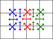 Additionally, there is an overlap in the pixel distances that are needed
for the current source pixel and those for the next source
pixel. Every source pixel uses five pixel distances that are shared with those
for the previous pixel. This brings the number of pixel distances to be
calculated down to 7 per source pixel. In the figure at the right of this
paragraph, the
blue and red arrows indicate the distances for the current pixel and
the red and green arrows those for the next pixel. The five red arrows
are thus the pixel distance calculations that are shared between the current
and next pixels.
Additionally, there is an overlap in the pixel distances that are needed
for the current source pixel and those for the next source
pixel. Every source pixel uses five pixel distances that are shared with those
for the previous pixel. This brings the number of pixel distances to be
calculated down to 7 per source pixel. In the figure at the right of this
paragraph, the
blue and red arrows indicate the distances for the current pixel and
the red and green arrows those for the next pixel. The five red arrows
are thus the pixel distance calculations that are shared between the current
and next pixels.
When considering implementation-specific optimization, specifically SIMD instructions, it is helpful to reduce the resolution of the bit-interleaved values. As implemented in the code snippet for bit interleaving, an interleaved value takes 24-bit. This is overly precise just to find an interpolation partner, especially because the difference between two interleaved values is only an approximate measure for the distance between the two colours. If we reduce this to 15-bit, by simply constructing the InterleaveTable differently, a subtraction between two such values fits in 16-bits. As already mentioned, the modern Intel processors can calculate the absolute value of four 16-bits values in parallel.
Another opportunity for optimization the code for magnifying by two is the series of if statements to find the minimum value. A sequence of CMP and CMOV instructions (Pentium-II processor and later) can calculate the mininum value without jumps (and thereby without penalties for mispredicted branches). SIMD instructions can help here too: Intel application note ([5]) describes the PMINSW instruction which determines the four minimum values of two groups of four 16-bit values. With three PMINSW instructions, plus some memory shuffling (hint: PSHUFW), we can find the four minimum values of four such groups.
And, like was the case for the minification algorithm, you might want to introduce extra local variables to avoid calculating the same values over and over again in the inner loop. Examples of such expressions in the magnify by two code are y*SrcWidth, y2*TgtWidth. Doing so immediately lets you simplify other inner-loop expressions such as (y2+1)*TgtWidth to Y2TgtWidth+TgtWidth, replacing a multiplication by an addition (the new variable Y2TgtWidth would be assigned the value of y2*TgtWidth at the top of the inner loop).
Currently the directionally averaging scaling algorithm only interpolates in one direction per target pixel, although that direction is linear. One additional rule, that might increase the quality of the result, is to use a bidirectional average if the maximum gradient is low. That is, in addition to the minimum gradient per target pixel, you also calculate the maximum value. If the maximum value is below some hard-coded limit, the target pixel gets the value of the average of four surrounding pixels.
Further reading
- [1] Riemersma, Thiadmer; "Quick and smooth image scaling with Bresenham"; Dr. Dobb's Journal; May 2002.
- A companion article, which describes the "smooth Bresenham" algorithm.
- [2] Riemersma, Thiadmer; "Quick colour averaging"; on-line article.
- A companion article, which describes how to calculate the (unweighted) average colour of two pixels in various formats.
- [3] Kientzle, Tim; "Approximate Inverse Color Mapping"; C/C++ User's Journal; August 1996.
- With bit-interleaving and a binary search, one obtains a palette index whose associated colour is close to the input colour. It is not necessarily the closest match, though, and the author already acknowledges this in the article's title. An errata to the article appeared in C/C++ User's Journal October 1996, page 100 ("We have mail").
- [4] Intel Application note AP-563; "Using MMX Instructions to Compute the L1 Norm Between Two 16-bit Vectors"; Intel Coorporation; 1996.
- The L1 norm of a vector is the sum of the absolute values. The note calculates the L1 norm of the difference between two vectors; i.e. it subtracts a series of values from another series of values and then calculates the absolute values of all these subtractions.
- [5] Intel Application note AP-804; "Integer Minimum or Maximum Element Search Using Streaming SIMD Extensions"; version 2.1; Intel Coorporation; January 1999.
- An algorithm to calculate the minimum value in an array considering four 16-bit words at a time.
- [6] Shezaf, N.; Abramov-Segal, H. Sutskover, I.; Bar-Sella, R.; "Adaptive Low Complexity Algorithm for Image Zooming at Fractional Scaling Ratio"; Proceedings of the 21st IEEE Convention of the Electrical and Electronic Engineers in Israel; April 2000; pp. 253-256.
- A follow-up on the article "Spatially adaptive interpolation of digital images using fuzzy inference" by H.C. Ting and H.M. Hang in Proceedings of the SPIE, March 1996.
- [7] Carrato, S.; Tenze, L.; "A High Quality 2× image interpolator"; Signal Processing Letters; vol. 7, June 2000; pp. 132-134.
- An algorithm to split a source pixel in 4 target pixels by looking at eight surrounding pixels. The algorithm is "trained" on a set of specific input images where the desired output for that image is known.
